NORFOX

Warning

This example is still under development; don’t read too closely yet.

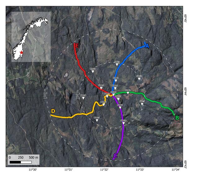
This example sketches a DASDAE inventory for the NORFOX fibre-optic array, a five-arm fiber-optic deployment at NORSAR’s Stendammen test site. The goal is to show how a complex public deployment can be represented by the DASDAE Inventory. Some liberties are taken with certain details, as the point of the exercise is demonstration, not exact accuracy.

Figure 1: NORFOX cable path and NORES stations, from the NORSAR NORFOX data page

This page is an illustrative inventory example for the proposal. It uses public NORFOX descriptions and an assumed local copy of the official KMZ. The exact Python API names may shift as the DASDAE inventory implementation evolves.

Source Material

The example assumes the official NORFOX KMZ has already been downloaded from the NORSAR page and placed locally:

data/NORFOX_interpolated_Arms.kmz

Each of NORFOX’s five arms is approximately 1700 m long, radiating from the Stendammen facility. Each arm contains an OCC 4x G652 standard fiber cable, an OFS AcoustiSense enhanced backscatter cable, and two empty 16 mm pipes. Arms C and E also include an empty 40 mm pipe. The cables are buried about 50 cm below the surface in forest soil. The OFS enhanced fiber is spliced to standard fiber at each arm end to close the loop. The deployment is co-located with the NORES seismic array.

Useful public references:

• NORFOX data page: https://www.norsar.no/data/norfox-fibre-optic-array-data
• Dataset DOI: https://doi.org/10.21348/d.no.0004
• Official KMZ: https://www.norsar.no/getfile.php/1319566-1696835035/KML%20filer/NORFOX_interpolated%20Arms.kmz
• NORSAR station network DOI: https://doi.org/10.21348/d.no.0001
• EIDA/FDSN data access: https://www.orfeus-eu.org/data/eida/webservices

Field Structure

The public arm layout can be summarized as follows.

Table 1: Public NORFOX arm structure represented in this example.

Arm	Approx. Length (m)	Fiber cables	Empty pipe enclosures	Notes
A	1700	OCC 4x G652, OFS AcoustiSense	2 x 16 mm	loop closure at arm end
B	1700	OCC 4x G652, OFS AcoustiSense	2 x 16 mm	loop closure at arm end
C	1700	OCC 4x G652, OFS AcoustiSense	2 x 16 mm, 1 x 40 mm	loop closure at arm end
D	1700	OCC 4x G652, OFS AcoustiSense	2 x 16 mm	loop closure at arm end
E	1700	OCC 4x G652, OFS AcoustiSense	2 x 16 mm, 1 x 40 mm	loop closure at arm end

Build The Inventory

The example uses a few constants and a local KMZ path. The coordinates in the KMZ are geographic, so the inventory CRS uses longitude, latitude, and elevation labels.

from pathlib import Path

import dascore.core.inventory as inv

KMZ_PATH = Path("data/NORFOX_interpolated_Arms.kmz")
ARMS = ("A", "B", "C", "D", "E")
ARM_LENGTH = 1700.0

crs = inv.CoordinateReferenceSystem(
    authority="EPSG",
    code="4979",
    name="WGS 84 3D",
    coordinate_labels=("longitude", "latitude", "elevation"),
    units=("degree", "degree", "meter"),
)

Interrogators

The NORFOX material identifies multiple interrogator configurations used for comparison. Interrogators are physical instruments, so they are modeled separately from acquisition streams.

Table 2: Interrogator configurations represented in the NORFOX example.

Interrogator	Role
Febus-A1R	DAS / phase-sensitive OTDR comparison
OptDAS	DAS / phase-sensitive OTDR comparison
OptDAS	DAS / phase-sensitive OTDR comparison

febus_a1r = inv.Interrogator(
    name="NORFOX Febus-A1R interrogator",
    manufacturer="Febus",
    model="A1R",
    instrument_type="DAS interrogator",
)
optdas_1 = inv.Interrogator(
    name="NORFOX OptDAS interrogator 1",
    model="OptDAS",
    instrument_type="DAS interrogator",
)
optdas_2 = inv.Interrogator(
    name="NORFOX OptDAS interrogator 2",
    model="OptDAS",
    instrument_type="DAS interrogator",
)

Acquisitions

Each interrogator configuration can produce its own acquisition stream while resolving to the same fiber array and optical paths. Wavelength-specific settings can be added later if they are needed for an analysis, but they are not required for the structural inventory.

common_acquisition_fields = dict(
    location_code="",
    data_category="DAS",
    data_type="strain_rate",
    data_units="1/s",
    start_distance=0.0,
)

febus_acquisition = inv.Acquisition(
    code="FEBUS",
    interrogator=febus_a1r,
    **common_acquisition_fields,
)
optdas_1_acquisition = inv.Acquisition(
    code="OPT1",
    interrogator=optdas_1,
    **common_acquisition_fields,
)
optdas_2_acquisition = inv.Acquisition(
    code="OPT2",
    interrogator=optdas_2,
    **common_acquisition_fields,
)

acquisitions = (
    febus_acquisition,
    optdas_1_acquisition,
    optdas_2_acquisition,
)

Cables And Pipe Enclosures

NORFOX is a good example of why container nesting is useful. Each arm has two fiber cables and multiple empty pipes. The cables and pipe enclosures are physical resources; the ordered optical path only contains components the light passes through.

def arm_resources(arm):
    occ_cable = inv.Cable(
        name=f"NORFOX Arm {arm} OCC 4x G652 cable",
        owner="NORSAR",
        manufacturer="OCC",
        model="4x G652",
        fiber_count=4,
    )
    ofs_cable = inv.Cable(
        name=f"NORFOX Arm {arm} OFS AcoustiSense cable",
        owner="NORSAR",
        manufacturer="OFS",
        model="AcoustiSense",
        fiber_count=1,
        diameter=0.0095,
        strength_member="Aramid Yarn",
        maximum_load=200,
        minimum_bend_radius=0.475,
    )
    pipe_enclosures = [
        inv.Enclosure(
            name=f"NORFOX Arm {arm} empty 16 mm pipe {index}",
            enclosure_type="pipe",
            inner_diameter=0.016,
        )
        for index in (1, 2)
    ]
    if arm in {"C", "E"}:
        pipe_enclosures.append(
            inv.Enclosure(
                name=f"NORFOX Arm {arm} empty 40 mm pipe",
                enclosure_type="pipe",
                inner_diameter=0.040,
            )
        )
    return occ_cable, ofs_cable, pipe_enclosures

Geometry From KML

The official KMZ contains one line for each arm. The proposed Geometry.from_kml helper lets the inventory import a named placemark without embedding thousands of coordinate rows in the example.

def arm_geometries(arm):
    outbound = inv.Geometry.from_kml(
        KMZ_PATH,
        label=f"Arm {arm}",
        name=f"NORFOX Arm {arm} outbound geometry",
        optical_length=ARM_LENGTH,
    )
    inbound = inv.Geometry.from_kml(
        KMZ_PATH,
        label=f"Arm {arm}",
        name=f"NORFOX Arm {arm} return geometry",
        optical_length=ARM_LENGTH,
        reverse=True,
    )
    return outbound, inbound

The intended behavior is:

• select the KML or KMZ placemark whose name matches label;
• import that placemark’s coordinate sequence using the inventory CRS;
• assign optical_length from the explicit argument;
• create a distance coordinate from 0 to optical_length along the imported sequence.
• reverse the coordinate sequence when reverse=True.

This keeps the example reproducible while still treating calibrated optical distance as inventory metadata, not something inferred blindly from map distance.

Optical Components

Each arm is represented with an enhanced DAS sensing cable, a splice at the arm end, and the standard fiber return path used to close the loop.

def arm_optical_components(arm, occ_cable, ofs_cable):
    enhanced_fiber = inv.FiberSegment(
        name=f"NORFOX Arm {arm} OFS AcoustiSense sensing fiber",
        optical_length=ARM_LENGTH,
        fiber_type="enhanced_backscatter",
        fiber_standard="OFS AcoustiSense",
        color="blue",
        attenuation_db_per_km=0.7,
        attenuation_wavelength=1550,
        rayleigh_backscatter_window=(1530, 1565),
        center_wavelength=1546,
        container=ofs_cable,
    )
    loop_splice = inv.Splice(
        name=f"NORFOX Arm {arm} loop closure splice",
        splice_type="fusion",
    )
    return_fiber = inv.FiberSegment(
        name=f"NORFOX Arm {arm} OCC G652 return fiber",
        optical_length=ARM_LENGTH,
        fiber_type="single_mode",
        fiber_standard="G652",
        color="white",
        attenuation_db_per_km=0.3,
        attenuation_wavelength=1550,
        container=occ_cable,
    )
    return enhanced_fiber, loop_splice, return_fiber

Coupling And Labels

The public installation description says the cables are buried about 50 cm below the surface in forest soil. That is an interval property, so it belongs on the coupling track.

def arm_couplings(arm):
    kwargs = dict(
        optical_length=ARM_LENGTH,
        coupling_type="trench",
        medium="forest_soil",
        attachment="direct_burial",
        depth=0.5,
    )
    return inv.CouplingCondition(**kwargs), inv.CouplingCondition(**kwargs)

def arm_annotation(arm):
    return inv.OpticalPathAnnotation(
        distance=0.0,
        optical_length=2 * ARM_LENGTH,
        label=f"arm_{arm.lower()}",
    )

Optical Paths

This example keeps each arm as a separate OpticalPath. That makes arm-level changes, outages, and repairs easy to represent over time. A different implementation could use one compound path with arm annotations if the acquisition stream is stored as one continuous channel axis.

optical_paths = []
physical_resources = []
for arm in ARMS:
    occ_cable, ofs_cable, pipe_enclosures = arm_resources(arm)
    physical_resources.extend((occ_cable, ofs_cable, *pipe_enclosures))
    path = inv.OpticalPath(
        name=f"NORFOX Arm {arm}",
        start_time="2022-01-01",
        optical_components=arm_optical_components(arm, occ_cable, ofs_cable),
        geometries=arm_geometries(arm),
        coupling_conditions=arm_couplings(arm),
        annotations=(arm_annotation(arm),),
    ).validate()
    optical_paths.append(path)

NORES Stations

The NORFOX deployment is co-located with NORES. The seismic array can live under the same network as conventional station/channel metadata while the fiber array carries the distributed optical paths.

Rather than manually transcribing station codes, coordinates, channels, and responses, the DASDAE inventory can ingest standard StationXML. ObsPy already knows how to read StationXML from the FDSN services, and the DASDAE layer can translate the standard station/channel objects into inventory Station and Channel objects. Response attachment is left as an exercise for the reader.

from obspy.clients.fdsn import Client

station_network_reference = inv.ExternalResource(
    uri="https://doi.org/10.21348/d.no.0001",
    name="NORSAR Station Network",
    description="Authoritative station metadata and citation for the NORSAR NO network.",
)
eida_access = inv.ExternalResource(
    uri="https://www.orfeus-eu.org/data/eida/webservices",
    name="UIB-NORSAR EIDA FDSN services",
    description="Waveform and StationXML access route for NORSAR NO network data.",
)

eida = Client("UIB-NORSAR")
nores_stationxml = eida.get_stations(
    network="NO",
    station="NR*",
    level="channel",
)

nores_stations = inv.Station.from_stationxml(
    nores_stationxml,
    include_response=False,
    notes="Co-located NORES seismometer imported from standard StationXML.",
)

physical_resources.extend((station_network_reference, eida_access))

The important point is that conventional seismic metadata should remain conventional. StationXML is already the exchange format for station coordinates, channels, epochs, and instrument responses; the DASDAE inventory only needs to attach the resulting stations beside the fiber array.

Assemble The Inventory

The fiber array uses a single observing identity for the NORFOX deployment and contains one path per arm.

fiber_array = inv.FiberArray(
    code="NORFOX",
    name="NORFOX fibre-optic array",
    acquisitions=acquisitions,
    optical_paths=tuple(optical_paths),
)

network = inv.Network(
    code="NO",
    name="NORSAR test site network",
    fiber_arrays=(fiber_array,),
    stations=nores_stations,
)

inventory = inv.Inventory(
    resources=tuple(physical_resources),
    coordinate_reference_system=crs,
    networks=(network,),
)

What This Example Exercises

NORFOX touches most of the model boundaries:

• KML-derived arm geometries are separate from calibrated optical distance.
• Two fiber cable types are represented as physical resources.
• Empty pipes are Enclosure resources with enclosure_type="pipe", not optical components.
• Loop closure is represented with ordered optical components.
• Burial in forest soil is represented as coupling context.
• NORES seismometers remain conventional station/channel metadata under the same network.